Philippine Earthquake Data for March to May 2016

In this activity, we are tasked to construct a network from earthquake data retrieved from Phivolcs [1] and compute the in-degree and out-degree distribution. We chose the March-May dataset as shown in Figure 1.

Figure 1. The nodes show the locations of detected earthquakes/tremors. The size of each node represents the magnitude while the colors represent the succession of events.

From these nodes, we construct a directed network based on the following rules:

1. All events are initially connected based on their temporal sequence.

2. The distances of an event to all the other events preceding it are calculated. The closest past event is then  connected to the to the current event being considered. 

The constructed networks based on these rules are shown in Figure 2.

Figure 2. Network constructed for the events in Figure 1 based on the rules outlined above.

In-degree and Out-degree Distribution

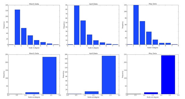
Figure 3. In-degree and out-degree distribution for the constructed networks

Figure 3 shows the in-degree and out-degree distribution for the networks. As expected, there are only three possible out-degrees: zero for the last node, one for a node when it is closest to its two otherwise. On the other hand, an in-degree of one is the most frequent among all three networks. This suggests that it is more probable for the next event to occur near the immediately succeeding event.

References:

1. Latest Earthquake Information. Retrieved from http://satreps.phivolcs.dost.gov.ph/index.php/earthquake/latest-earthquake-information

Collaborators:

Mary Angelie M. Alagao

Maria Eloisa M. Ventura

2D Cellular Automata: Three-state Majority Rule

In the previous post I've shown the evolution of elementary cellular automata (CA) for different rules. Now we'll go to the next step and check out a 2D cellular automata model. Just as in 1D CA, the value of a cell in a 2D CA model is dictated by its neighbors. However, for 1D CA a cell only has two neighbors whereas for a 2D CA a cell can have either four or eight neighbors depending on the neighborhood type we are considering. 

So what are these neighborhood types? There are two:

Neighborhood Types

1. Moore neighborhood

The Moore neighborhood consists of the eight cells surrounding a central cell in a 2D lattice. The figure below shows an illustration of the Moore neighborhood. 

2. Von Neumann neighborhood

The Von Neumann neighborhood is comprised of the four cells orthogonal to a central cell as shown in the image below.

Figure 1. The blue cells indicate the neighbors of the central cell (orange cell)
for the Moore neighborhood (left) and the Von Neumann neighborhood (right) 

There are several 2D cellular automata models that are currently used to model systems, such as the simple binary majority rule, Conway's Game of Life, the Schelling model, Turing patterns, and the Sandpile model. 

Majority Rule

For this post we'll be dealing with the simplest of these: the majority rule. As the name of the model suggests, the value of a cell is updated depending on which state is most dominant among its neighbors. Here, we model a three-state system with a Moore neighborhood starting with an initially random distribution of states and letting the system evolve in time while taking note of the following rules:

1. When there exists a dominant state $S_{maj}$ among the three states $S = {0, 1, 2}$ in the neighborhood, the value of the central cell is updated to $S_{maj}$.

2. In case there is no clear dominant state (i.e. in case of a tie in the frequency of some states) in the neighborhood then the value of the central cell is unchanged.

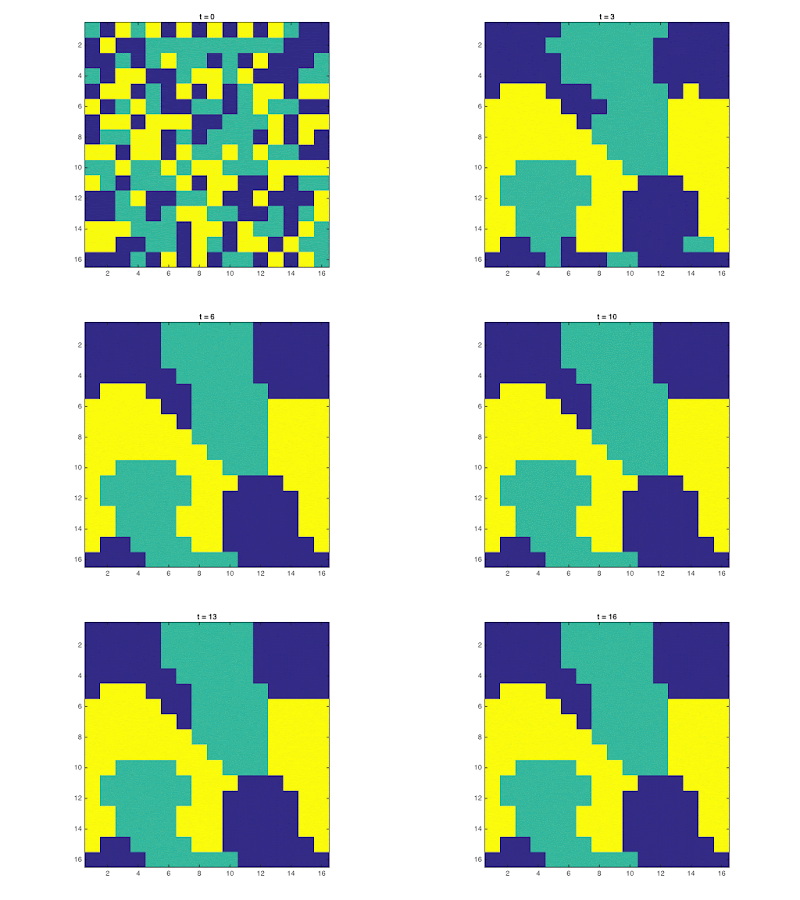
Shown below are snapshots of the 2D lattice over several iterations for different lattice sizes.

Evolution of an 8x8 lattice for three-state majority rule

Evolution of a 16x16 lattice for three-state majority rule

Evolution of a 32x32 lattice for three-state majority rule

Evolution of a 64x64 lattice for three-state majority rule

It can be observed, especially for $N>8$,  that as the system evolves it reaches a steady state. From the considered systems, it is possible to achieve a "unanimous" state in which all cells have equal values or a steady state in which no clear majority exists in the Moore neighborhood of all cells so the system no longer evolves and stays in this state. 

Collaborators:

Mary Angelie M. Alagao

Maria Eloisa M. Ventura

BTW Sandpile Model

One of the things most of us loved to do in the beach as children (or maybe even as adults?) was to play with sand. We put grains of sand on top of each other and sometimes get frustrated when the pile topples. 

So, why do the grains of sand to topple? And when do they topple?

Initially, we have a random distribution of sand over a finite space. Adding more grains of sand causes the slope of the pile to become steeper. Some sites become more unstable than others such that they can no longer hold any more grains and any additional grain will simply tumble down the pile. Sometimes, the pile reaches a state in which a single grain that is tumbling down may carry others with it, causing a large-scale avalanche. We may technically call this a critical state of the sandpile. Seeing as the criticality arose without tuning any parameters, this phenomenon is called self-organized criticality (SOC), a concept which was first suggested by Per Bak, Chao Tang and Kurt Wiesenfeld in their 1987 paper [1]. The concept of SOC is now widely applied across different fields.

In the same paper they introduced the Bak-Tang-Wiesenfeld (BTW) sandpile model which is one of the dynamical systems that exhibited SOC. The BTW model is also an example of a 2D cellular automaton.

Algorithm

In this activity, we implemented the BTW sandpile model using the following algorithm:

1. Initialize random $N \times N$ array $A$ with possible states $S = {0, 1, 2, 3}$.
2. Iteration{
• Randomly select a site (i, j) and update the state of the cell by adding 1, i.e. $S_{t+1} = S_{t} + 1$.
• Check whether the state of the cell (i, j) satisfies $A_{ij} \ge 4$
• i. If Yes: Then the site is unstable and it can topple its "contents" to its four neighbors (i.e. Von Neumann neighborhood) so you update the values of the cells to:
• $A_{ij} \longrightarrow A_{ij} - 4$
• $A_{i-1,j} \longrightarrow A_{i-1,j}  + 1$
• $A_{i+1,j}\longrightarrow  A_{i+1,j}  + 1$
• $A_{i,j+1} \longrightarrow  A_{i,j +1} + 1$
• $A_{i,j-1} \longrightarrow  A_{i,j -1} + 1$

• If No: Proceed to next iteration
• Check the neighborhood for other unstable sites and repeat the toppling process until all sites are stable before proceeding to the next iteration. 
• Note: There are sinks along boundaries of the grid so for cells along the edge that topple  the grains are "thrown" in the sinks.}

In our implementation, a 128 x 128 array was used and the system was allowed to evolve for T = 100, 000 iterations. In each iteration, we take note of the the avalanche size or the number of cells affected by the the toppling due to a cell's instability.

Results

The time series for the avalanche sizes is shown in Figure 2. It can be observed that at around t ~30,000, the system enters its critical state. The reaction of the system to small perturbations becomes highly nonlinear, resulting to high uncertainties in the outcome of the the disturbance. The effect of the perturbation ranges from small shifts to a global avalanche depending on where the perturbation is applied. In the sandpile analogy, addition of a "grain of sand" can either cause a global avalanche or small rearrangements in the distribution of sand in localized regions.  This is a manifestation of the system's self-organized criticality.

Figure 2. Time series for the avalanche sizes

The animations below show the behavior of the system before and after it achieved its critical state. These images show the sandpile before the cells are updated in case of an avalanche. The images show that when the system reaches its critical state the sandpile become dense.

(a) Before reaching critical state

(b) After reaching critical state

Figure 3. Animations showing the bahavior of the system (a) before and (b) after reaching the critical state 

We also examine the distribution of the avalanche sizes, shown in Figure 3 in logarithmic scale. The linear trend suggests a power-law size distribution which is characteristic of SOC. From the fit, the power law exponent of the system is $\alpha = -1.195$.

Figure 4. Distribution of avalanche sizes

References:
1. Bak, Per, Chao Tang, and Kurt Wiesenfeld: Self-organized criticality: An explanation of the 1/f noise. Phys. Rev. Lett., 59(4):381–384, Jul 1987.
2. S. Lübeck and K. D. Usadel., Bak-Tang-Wiesenfeld sandpile model around the upper critical dimension.  Phys. Rev. E 56, 5138 (1997).


Collaborators:

Mary Angelie M. Alagao

Maria Eloisa M. Ventura

Fractals

Sometimes when you're sitting in your higher Mathematics class you feel like there isn't really any connection between what you're learning and the real world out there. Especially when you look at the board filled with those seemingly meaningless symbols. What we often forget is that Mathematics is all around us. The natural world is filled with patterns: from the structure of a spider's web, the meandering rivers, the shape of honeycombs, and even the shape of a snowflake. All these can be described by Mathematics.

One of the interesting phenomena we see in nature is the existence of fractals. These are objects or quantities that exhibit self-similarity on all scales. When you zoom in on a fractal structure you will see a similar pattern each time, making it seem never-ending. Examples of fractals are the Koch snowflake, the Mandelbrot set, and the Serpinski sieve [1]. There are also many objects in nature that are fractals such as the repeating patterns in peacock feathers, in ferns and in trees. 

One way to describe a fractal is by quantifying its fractal dimension which gives an idea on the complexity of a curve's geometry [1]. Unlike the spatial dimensions that we are used to, the fractal dimension is a non-integer.

In this post we will determine the fractal dimension of a fractal using the box-counting method. In this technique we set a box size and count the non-zero cells in the box while sliding it across the image of the fractal. We do this for several box sizes and plot the box count versus the inverse of the box size in logarithmic scale and find the slope of the trend line to get the fractal dimension $\epsilon$.

Here, we try to determine the fractal dimension of a neuron as shown in the figure below.

Figure 1. Image of a neuron and its binarized version (Image taken from [2])

From Figure 2, the fractal dimension of the neuron is equal to 1.5898.

Figure 2. Plot of the box count versus box size in logarithmic scale

References:
1. Fractals. Retrieved from http://mathworld.wolfram.com/Fractal.html on June 5, 2016
2. Image retrieved from https://www.nikoninstruments.com/About-Nikon/News-Room/US-News/Neuroscientist-and-Founder-of-the-Nikon-Microscopy-Center-of-Excellence-in-Budapest-Featured-in-Tech-Heroes-Campaign-on-CNN.com

Properties of an Erdos Renyi Network

The Erdos Renyi (ER) Network is a random graph model. In this type of network, the nodes are connected based on a random probability, $p$, of an edge existing. ER graphs are characterized by a binomial degree distribution which at very large $N$ approaches the Poisson distribution. ER Network is useful when one has an absolute lack of knowledge in the principles governing edge creation. 

An ER Network has the following properties at large N:

1. As $N \rightarrow \infty,  <K> = Np$

2. As $N \rightarrow \infty,  <C> = p$

3. As $N \rightarrow \infty$, the degree distribution approaches a Poisson distribution

For this post, we'll be showing these notable properties of of an ER network. We construct an ER network with varying lattice sizes and determine whether we get the above quantities for very large $N$. 

The outline for the network construction is as follows:

1. We initialize a random $N \times N $ lattice A with values ranging from. We set a threshold  $th  \epsilon [0,1]$ which determines whether two nodes will be connected. When $A_{ij} \ge th$ then we change its value to 1 otherwise we change it to 0. Hence the probability of an edge existing is given by $p = 1 - th$.

2.  We construct the adjacency matrix and use it to solve for the mean degree, $<K>$, mean clustering coefficient, $<C>$, and the degree distribution for several degree sizes.

Shown below are the plots of the degree distribution for increasing values of $N$. The mean degree, $<K>$ and the %error from the mean of a Poisson distribution $\lambda = Np$. As shown by the decreasing %error, $<K>$ approaches $\lambda = Np$ as the number of nodes become large.

Figure 1. Degree distribution for different number of nodes N in the ER network

The summary of the network metrics are shown in Table 1. It can be observed that as N increases the errors in the quantities also decrease, suggesting that the values for <K> and <C> reduce to $Np$ and $p$ for large $N$, respectively. 

Table 1. Summary of network metrics ($<K> $- average degree,$ <C> $average clustering coefficient, $M $ number of edges) for different number of nodes $N$ in an Erdos-Renyi network